
These line graphs represent references to God found within inaurual addresses from George Washington's first address in 1793 to Barack Obama's address in 2013. The first graph displays the total references found within the speeches. In essence this graph shows the sum of all supplication, humility, testimony, and praise references found within the speeches. We looked for any correlation between the amount and type of references with the political and social climate of the nation at the time. As we expected, there were instances of increased references to God during periods of national strife such as the War of 1812 and the Civil War. Suprisingly, however, during other tumultuous times such as the Great Depression and the inaugural address given by George W. Bush in 2004, the first address following the attacks of September 11, the amount of references actually went down.
This graph displays the total amount of God terms found within inaugural speeches over the course of American history. Within each reference, there may be more than one use of a God term. This could be multiple pronouns, or multiple examples of the actual word God. What is interesting about this graph is the spike found in Abraham Lincoln’s second inaugural address. This address was given in 1865 following four years of terrible civil war within the United States. This can be construed as an example of references to God going up during times of national strife. Another spike in the amount of God terms occurs in Ronald Reagan’s second inaugural address. This address was given during the Cold War, a time when the United States emphasized its Judeo-Christian background as opposed to the state atheism of the Soviet Union.
In short, regression analysis is a statistical method to estimate the relationship between a dependent variable (commonly referred to as “y” or the left side variable) and one or more independent variables (commonly referred to as "x" or the regressors). Regression analysis provides a model that allows a user to gain understanding of how the typical dependent variable changes with changes in the independent variables, holding the other independent variables constant. Because of this functionality, regression is typically used to predict or forecast the value of the dependent variable, when values for the independent variables are known.
There are different types of regression models depending on the nature of the data. The simplest type of regression model is a standard linear model. This method may be familiar to a user who have done basic line of best fit work with scatter plots, as seen below.
Of course, whenever you include more than one variable and change the characteristics of the predicted variable, the more complicated a model one has to use for accurate results. For example, in the previous illustration the dependent variable was weight—which is a continuous variable (theoretically one could weigh 110 pounds, 110.0001 pounds, 110.0002 pounds…), but what if the dependent variable was a discrete counting number? For our project, our dependent variable—the number of references to God—is a discrete variable for it can have the value 1, 2, 3… but a speech cannot have 1.467 references to God. The Poisson regression model is usually used on data of the counting nature.
One of the primary differences between a simple linear regression model, and a Poisson regression model is what is called the “link function.” A link function is what links the independent variables to the error term. In the standard linear regression, the link function is an identity link, meaning that the coefficients or the “slope terms” can be interpreted as seen above. The link function for the Poisson model is much more complex, with the use of logarithmic functions. The model will be further explained with an applied approach with the data collected.
In pure mathematical terms: a one unit change in the independent variable, e.g. the increase of one child, other variables held constant, results in the difference in the logs of the expected counts in the amount of the regression coefficient of that variable. In equation terms:
Where β is the regression coefficient, μ is the expected count of the dependent variable, denoting a one unit increase.
Using rules of logarithms, a term called the incident rate ratio (IRR), which has a more direct interpretation as seen in the simple regression model, can be calculated from the Poisson regression coefficients. More information on the Poisson regression model can be found here.
Our dependent variable was the average number of references to God used by a President, with the President's background information as the independent variables. For background on the variables used in our Poisson regression, check out the regression codebook. The nature of our data required the frequent use of binary or dummy variables, which are qualitative variables. A "female" dummy variable would take a value of 1 if the individual was a female, 0 if the individual was a male.
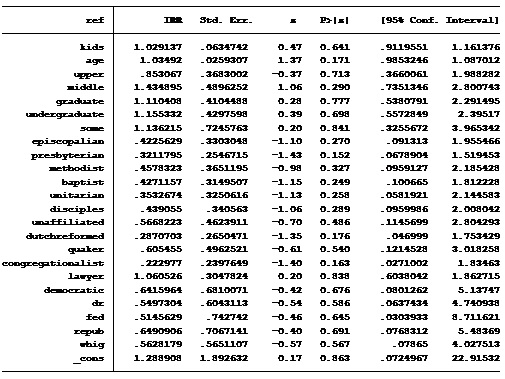
The actual statistical mathematics required to produce the Poisson model was done in the STATA software which is free to all University of Pittsburgh students. Upon running the regression, a slightly dissappointing, yet still informative statistic was revealed. The probability of getting the null hyptothesis, i.e. the probability of all of the regressors being statistically insignificiant and having no significant effect, was 99.4%. Therefore, one could conclude that the variables in our study including the President's age, number of kids, religious denomination, political party, and profession do not seem to have a statistically significant effect. This is not to say that there exist no variables that could predict a President’s use of references to God, but one would have to look elsewhere! At the same time, 39 individual Presidents, truly is a small sample size, so measurable statistics may have to wait for American democracy to grind on for a while.
Below the STATA output of the hypothetical IRR values are provided. For the sake of knowledge, an IRR value from the Poisson model can be interpreted as: for a one-unit increase in a variable (say 1 more kid, all other variables constant) a President is 1.0291 times more likely to reference God. But once again, these values are insignificant—even on an individual basis as the P > [z] values are all extremely high.

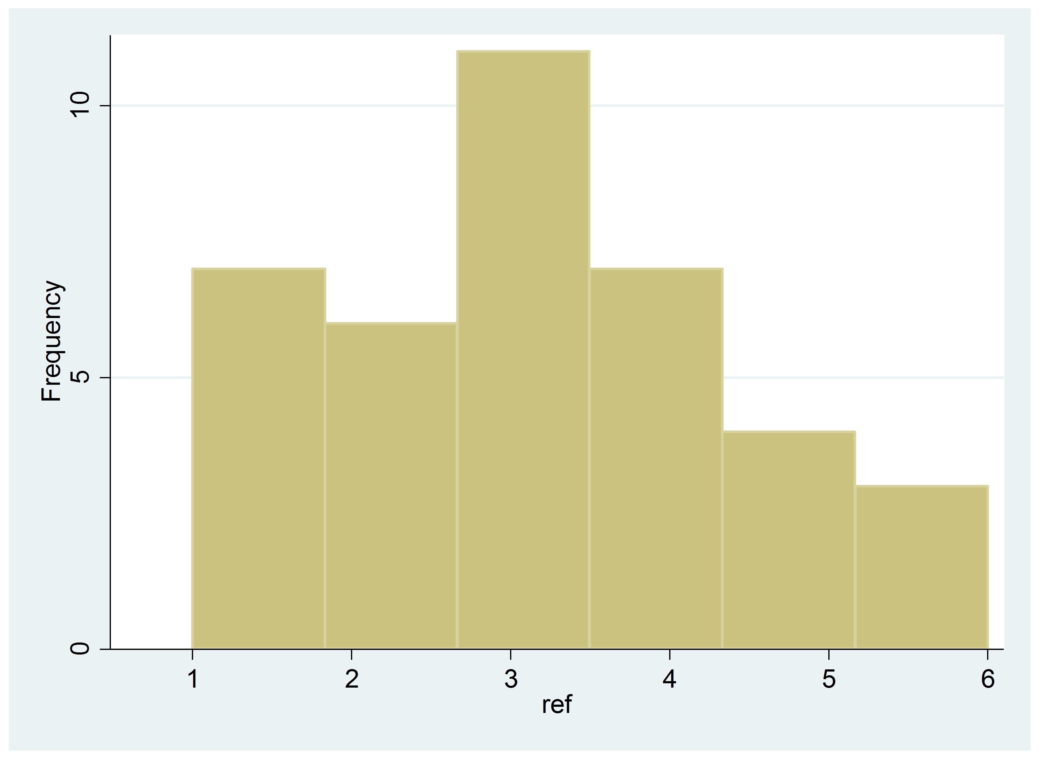
Here is a histogram of the amount of references to God per address. This histogram looks extremely similar to a standard normal distribution, a distribution that is common among random variables. I am definitely not going as far to say that the number of references to God is a random variable, but potential future research on this project would be interesting to examine that possible distinction.
